Two-, three sites mixed enzyme inhibition
Redirected from the LMx(Sp>Ca)I page, study by Lorey et al. [1]. When three modifier molecules (X) bind the enzyme in three different ways (Scheme 1), the denominator of the rate equation contains additional terms. The mechanism has been called parabolic mixed-type inhibition because the dependence of (Km/kcat)app on modifier concentration is described by a curved up parabola.
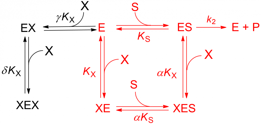
Scheme 1 is an extension of the general modifier mechanism, to which a two-step, dead-end branch leading to a catalytically inactive complex XEX has been added. The reactions paths in red correspond to linear mixed inhibition that can be either predominantly specific, predominantly catalytic or balanced. The addition in compulsory order of two modifier molecules to free enzyme (black reaction paths) that lead to the dead-end complex XEX introduce an [X]2 term in the rate equation:
(1) ![\begin{equation*} \ratev = \dfrac{{V\left[ {\rm{S}} \right]}}{{{K_{\rm{m}}}\left( {1 + \dfrac{{\left[ {\rm{X}} \right]}}{{{K_{\rm{X}}}}} + \dfrac{{\left[ {\rm{X}} \right]}}{{\gamma {K_{\rm{X}}}}} + \dfrac{{{{\left[ {\rm{X}} \right]}^2}}}{{\gamma \delta {\mkern 1mu} K_{\rm{X}}^2}}} \right) + \left[ {\rm{S}} \right]\left( {1 + \dfrac{{\left[ {\rm{X}} \right]}}{{\alpha {\mkern 1mu} {K_{\rm{X}}}}}} \right)}} \end{equation*}](https://www.enzyme-modifier.ch/wp-content/ql-cache/quicklatex.com-9a7721d6b6f8546654c4db80767539e6_l3.png "Rendered by QuickLaTeX.com")
The term parabolic refers solely to the shape of (Km/kcat)app on modifier concentration and should not suggest a behavior different from any linear-type inhibition. In fact, linear refers to reactions in which the rate is driven to zero at saturating inhibitor concentration, which is the case in equation (1).
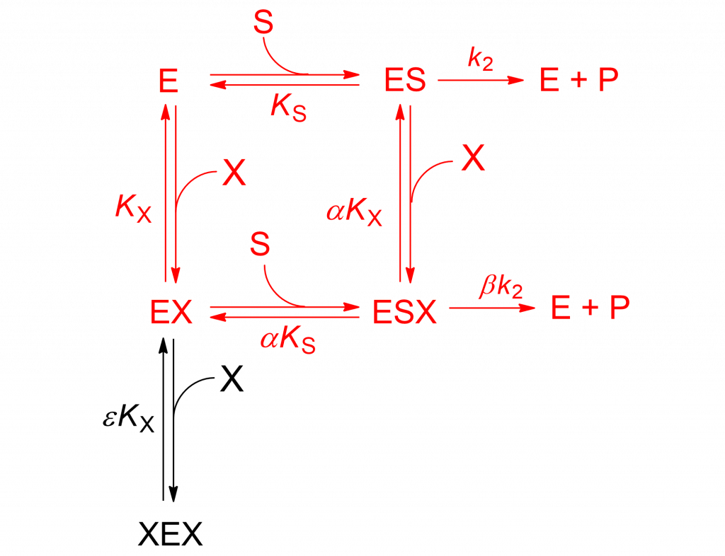
(2) ![\begin{equation*} \ratev = \dfrac{{V\left[ {\rm{S}} \right]}}{{{K_{\rm{m}}}\left( {1 + \dfrac{{\left[ {\rm{X}} \right]}}{{{K_{\rm{X}}}}} + \dfrac{{{{\left[ {\rm{X}} \right]}^2}}}{{\varepsilon K_X^2}}} \right) + \left[ {\rm{S}} \right]\left( {1 + \dfrac{{\left[ {\rm{X}} \right]}}{{\alpha {K_{\rm{X}}}}}} \right)}} \end{equation*}](https://www.enzyme-modifier.ch/wp-content/ql-cache/quicklatex.com-7d3b3ce5c00952b51d671fadf40a4195_l3.png "Rendered by QuickLaTeX.com")
The mechanism in Scheme1 is analogous to the two-sites mixed modification model shown in Scheme 2, discussed in detail in [2, pp. 191-198]. With β = 0 the rate equation becomes:
(3)
References
- Lorey S, Stöckel-Maschek A, Faust J, Brandt W, Stiebitz B, Gorrell MD, Kähne T, Mrestani-Klaus C, Wrenger S, Reinhold D, Ansorge S, Neubert K (2003) Different modes of dipeptidyl peptidase IV (CD26) inhibition by oligopeptides derived from the N-terminus of HIV-1 Tat indicate at least two inhibitor binding sites. Eur J Biochem 270: 2147-2156. doi:10.1046/j.1432-1033.2003.03568.x
- Baici A (2015) Kinetics of Enzyme-Modifier Interactions – Selected Topics in the Theory and Diagnosis of Inhibition and Activation Mechanisms. Springer, Vienna