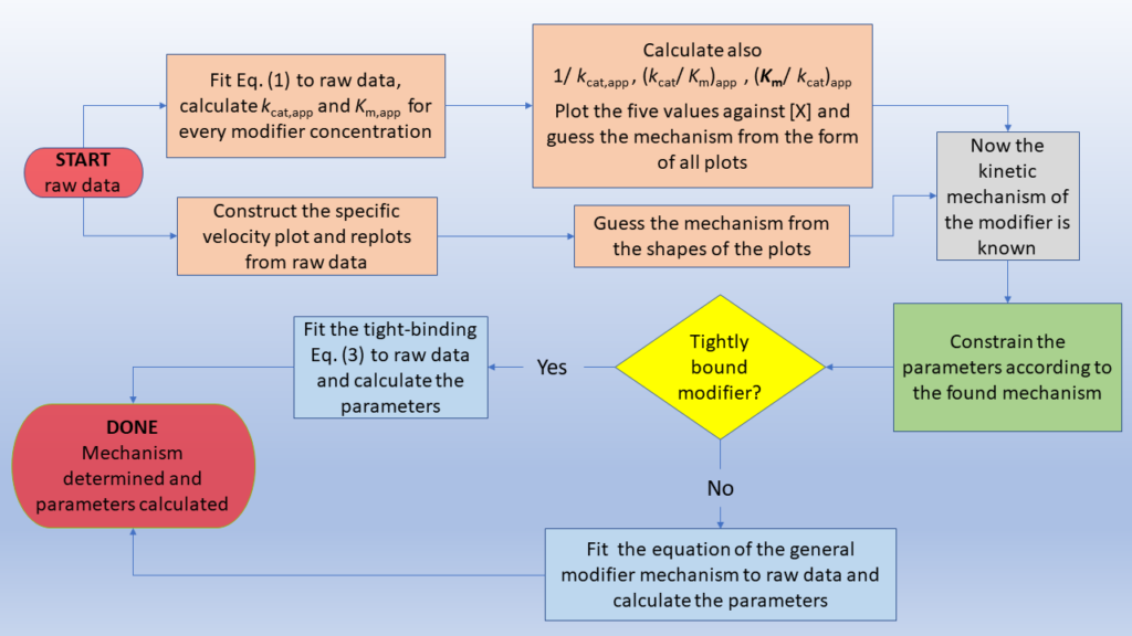
From raw data to the mechanism
This tutorial section is aimed at suggesting a logical way that leads from raw enzyme kinetic data to the identification of the mechanism and to the calculation of the sought kinetic parameters. After commenting the required quality of raw data, two strategies that can be applied individually or, better, in combination, will be discussed for determining the basic kinetic mechanism of modification before using any equation for calculating the kinetic parameters. The first method exploits the dependence of the kinetic parameters on modifier concentration, and the second is a graphical approach that uses the specific velocity plot.
In the final polish, the information gathered from either one or both preceding steps is mandatory for choosing the appropriate equation and parameter constraints for reanalyzing the raw data and calculating the parameters. Any tight-binding condition between enzyme and modifier can be taken into account to overcome the problem of modifier depletion. Below an overview of the topics of this section.
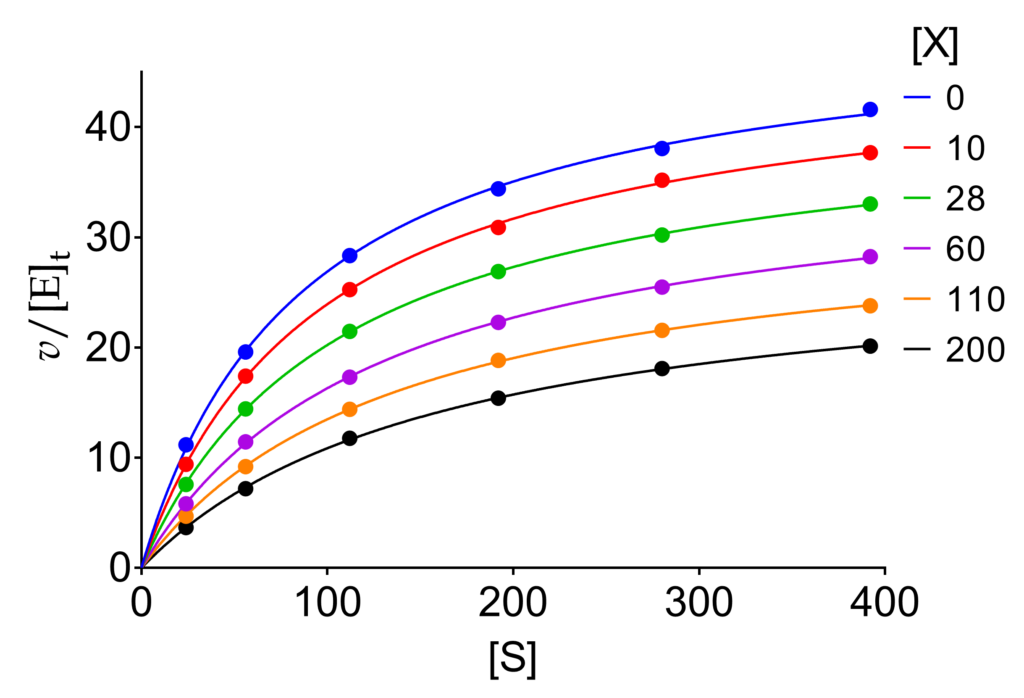
In Fig. 1, the equation fitted to raw data is the general modifier mechanism equation written in a condensed form that resembles the Michaelis-Menten equation (1). The superscripts highlight the fact that, in the the presence of a modifier, the parameters become apparent.
(1) ![\begin{equation*} \dfrac{v}{{{{\left[ {\rm{E}} \right]}_{\rm{t}}}}} = \dfrac{{k_{{\rm{cat}}}^{{\rm{app}}}\left[ {\rm{S}} \right]}}{{K_{\rm{m}}^{{\rm{app}}} + \left[ {\rm{S}} \right]}}\ \end{equation*}](https://www.enzyme-modifier.ch/wp-content/ql-cache/quicklatex.com-68154b7da3f5d5cbf1a5611d334303a7_l3.png "Rendered by QuickLaTeX.com")
The magic of (1) is its ability to fit rectangular hyperbolas and to catch changes of kcat and Km depending on the mechanism (α and β), and modifier concentration [X]. The explicit expressions of the apparent parameters are shown in (2).
(2) ![\begin{equation*} k_{\text{cat}}^{\text{app}}={{k}_{2}}\times \dfrac{1+\beta \dfrac{\left[ \text{X} \right]}{\alpha {{K}_{\text{X}}}}}{1+\dfrac{\left[ \text{X} \right]}{\alpha {{K}_{\text{X}}}}}\qquad {K}_{\text{m}}^{\text{app}}={{K}_{\text{m}}}\times \dfrac{1+\dfrac{\left[ \text{X} \right]}{{{K}_{\text{X}}}}}{1+\dfrac{\left[ \text{X} \right]}{\alpha {{K}_{\text{X}}}}} \end{equation*}](https://www.enzyme-modifier.ch/wp-content/ql-cache/quicklatex.com-ce878ed1327c6d11d7de0155949fef68_l3.png "Rendered by QuickLaTeX.com")
Raw data analysis step-by-step
Parameter dependence on modifier concentration
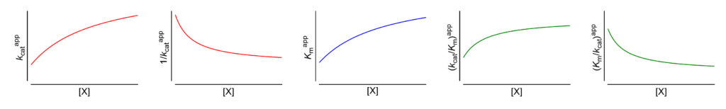
After extracting the apparent values of kcat and Km from raw data (see above), the dependence of kcat, 1/kcat, Km, kcat/Km and Km/kcat on [X] is analyzed. There are 17 physically meaningful patterns, one each for the 17 basic modifier mechanisms, which can thus be determined unequivocally.
Parameter dependence on [X] step-by-step
The specific velocity plot
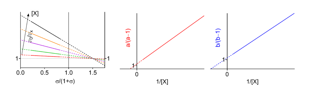
Using the raw data, the v0/vX ratios (velocity in the absence of modifier divided by the velocity in its presence) are calculated for all substrate and modifier concentrations and plotted against the specific velocity σ/(1+σ), where σ = [S]/Km. Secondary plots from the intercepts of the lines with the ordinates at the abscissa values 0 (a) and 1 (b) are then constructed. The mechanisms of enzyme modification can be determined by inspection of the graphics. The specific velocity plot, grounded on the general modifier mechanism, applies to all seventeen basic modifier mechanisms, each one with its own, unique graphical patterns.
The specific velocity plot step-by-step
The final polish
In this website, lets us agree that when we talk about enzyme-modifier interactions without further adjectives or specification, we intend that a tight-binding interaction between enzyme and modifier is not present.
The safest way to calculate the kinetic parameters of enzyme modifiers is first to determine the kinetic mechanism, to constrain, accordingly, one or more of the parameters to a fixed value, and then to fit the equation of the general modifier mechanism with constrained parameters to raw data. The policy of direct fit of a limited set of equations to data, e.g. the classical equations for linear competitive, uncompetitive and mixed inhibition, can or cannot be successful because these three equations can identify just a subset of the seventeen existing mechanisms.
Why should we always think only at inhibition, and what about nonessential activation? Do you know that inhibition detected at a given substrate concentration can turn into activation just by increasing the substrate concentration, and that this is an important regulatory mechanism in the metabolism of fatty acids? Why not abandon obsolete methods that produced and continue to produce a plethora of mistakes in the literature?
The final polish for tightly-bound modifiers
Tight-binding of a modifier (X) to an enzyme (E) is merely an experimental issue. If velocity measurements are performed at comparable concentrations of E and X and these concentrations fall in the range of the dissociation constant of the EX complex, a non-negligible portion of modifier is bound to the enzyme thus invalidating the condition [X]free ≈ [X]total. The following equation (3) overcomes this problem allowing to calculate the relevant kinetic parameters without bias.
(3) ![\begin{equation*} {\ratev_{\rm{X}}} = \dfrac{{{\ratev_{\rm{0}}}}}{2}\left[ {1 - \dfrac{{\beta \left( {1 + \sigma } \right)}}{{\alpha + \sigma }}} \right]\left\{ \begin{array}{l} \sqrt {\left[ {{{\left( {\dfrac{{1 + \sigma }}{{\alpha + \sigma }}\dfrac{{\alpha {K_{\rm{X}}}}}{{{{\left[ {\rm{E}} \right]}_{\rm{t}}}}} + \dfrac{{{{\left[ {\rm{X}} \right]}_{\rm{t}}}}}{{{{\left[ {\rm{E}} \right]}_{\rm{t}}}}} - 1} \right)}^2} + 4\dfrac{{1 + \sigma }}{{\alpha + \sigma }}\dfrac{{\alpha {K_{\rm{X}}}}}{{{{\left[ {\rm{E}} \right]}_{\rm{t}}}}}} \right]} + \dfrac{{\alpha + \sigma + \beta \left( {1 + \sigma } \right)}}{{\alpha + \sigma - \beta \left( {1 + \sigma } \right)}} - \dfrac{{1 + \sigma }}{{\alpha + \sigma }}\dfrac{{\alpha {K_{\rm{X}}}}}{{{{\left[ {\rm{E}} \right]}_{\rm{t}}}}} - \dfrac{{{{\left[ {\rm{X}} \right]}_{\rm{t}}}}}{{{{\left[ {\rm{E}} \right]}_{\rm{t}}}}} \end{array} \right\}\ \end{equation*}](https://www.enzyme-modifier.ch/wp-content/ql-cache/quicklatex.com-f3155b059ed3d3648005ed2ad5a7feb6_l3.png "Rendered by QuickLaTeX.com")
Don’t panic for this apparently complicated equation: it is very friendly for nonlinear regression purposes and can even be used as default for any mechanism, also when the tight binding condition is not present.
Tightly-bound modifiers step-by-step