The worked example discussed here is the same as in the preceding pages. The data, simulated by adding error, are very useful for comparing the results with the theoretical values, considering or not constrained parameters.

The plots discussed under Raw data illustrated the information that can be gathered from the dependence of the kinetic parameters on modifier concentration. Fitting the appropriate equations to the values of k_cat, K_m and k_cat/K_m yielded fairly good estimates of the parameters that serve to identify the mechanism, notably α and β. Figs. 2 and 4 in the page Raw data afforded α = 2.4 and β  = 0.4, sufficient to assert that the data belong to a hyperbolic mixed,  predominantly specific inhibition mechanism, acronym HMx(Sp>Ca)I. The same diagnosis was obtained using the dependence of the kinetic parameters on modifier concentration and the specific velocity plot.

We wish now to refine the calculation of the parameters using the entire set of raw data. To this end we fit eq. (1) to the data in Table 1 globally sharing the parameters among the six curves. The plots are shown in Fig. 1.

 (1)    

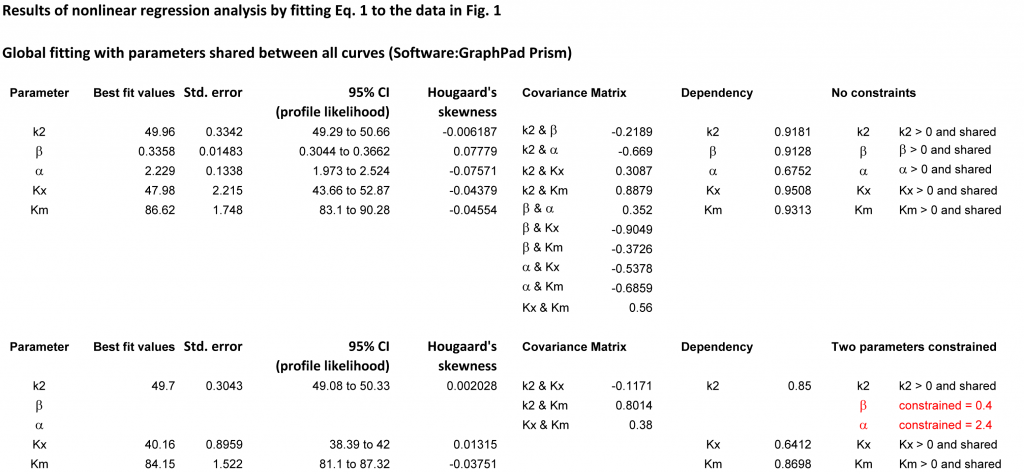
In the results table it is important to examine not only the parameters with their errors and confidence intervals but also the dependency of each parameter from the remaining parameters. Table 2 reports a summary of the fits, while Table 3 shows more details, such as the covariance matrix.

In Table 2, column 1, all parameters were included unconstrained in the fit. K_X has the largest deviation from the theoretical value and the strongest dependency from the other parameters. The normalized covariance matrix of β and K_X is in this case −0.9049, the largest among all combinations of parameters (Table 3). This suggests that constraining  β and possibly at least another parameter may improve the quality of the procedure.

Considering Table 2, constraining only α (column 2) or only K_m (column 3) has minor on no benefits. However, constraining β (column 4) or α and β at the same time (column 5) produces a trustworthy value of K_X. Thus, global analysis, constraining α and β is a good method for estimating the other parameters. Their deviation from the unknown true values depends on the quality of raw data.

To identify the parameter that causes a large dependency, the covariance matrix can be examined. Unlike the dependency, which is a single value calculated for each parameter, the covariance matrix provides the normalized covariance for all pairs of parameters in the model and has values between −1 and 1. When the dependency is high, the normalized covariance with at least another parameter is high as well.

Dependency and covariance matrix: practical hints

Adapted from GraphPad Prism, Curve Fitting Guide (once in the website search for dependency ).

The dependency varies between 0 and 1 and states how much a given parameter is intertwined with all remaining parameters. Completely independent parameters have a dependency of 0, while a dependency of 1 indicates that the parameters are redundant. With a high dependency, the same curve can be created with different sets of parameter values.

Remedies: 1) a simpler model can possibly perform better; 2) two or more  sets of different experiments can be analyzed by global fitting; 3) constrain critical parameters to constant values if these can be determined independently.

Table 1. Raw data of the initial velocities in Fig. 1 as v/[E]_t

[S]	[X] = 0	[X] = 10	[X] = 28	[X] = 60	[X] = 110	[X] = 200
24	11.18	9.40	7.57	5.82	4.70	3.67
56	19.60	17.40	14.43	11.44	9.19	7.19
112	28.34	25.26	21.46	17.32	14.40	11.76
192	34.41	30.89	26.90	22.27	18.82	15.40
280	38.05	35.18	30.21	25.47	21.56	18.08
392	41.60	31.67	33.02	28.24	23.79	20.12

---

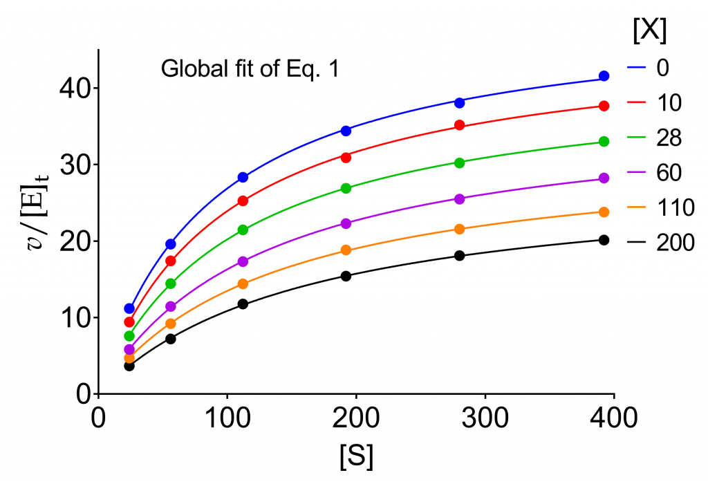
Table 2. Summary of the best-fit results from fitting (1) to the data in Table 1/Fig. 1. Numbers in parentheses represent the dependency of the considered parameter from the remaining parameters. In rows 2-5, the red numbers indicate the parameters that were constrained to fixed values in order to appreciate how the remaining fitted parameters change in comparison with their theoretical values. Original results in Table 3 with a complete list. The redundant precision with two decimals serves merely to illustrate the method.

	1	2	3	4	5	6
Parameter	No constraints	α constrained	Km constrained	β constrained	α and β constrained	Theor. values
α	2.23 ± 0.13 (0.6752)	2.4 (1)	2.21 ± 0.09 (0.3912)	2.5 ± 0.2 (0.4283)	2.4 (1)	2.4
β	0.34 ± 0.01 (0.9128)	0.34 ± 0.01 (0.9007)	0.33 ± 0.09 (0.8991)	0.40 (2)	0.40 (2)	0.35
k2	49.96 ± 0.33 (0.9181)	49.69± 0.25 (0.8499)	50.03 ± 0.15 (0.6129)	49.53 ± 0.39 (0.908)	49.7 ± 0.3 (0.85)	50
KX	47.98 ± 2.22 (0.9508)	46.63 ± 1.83 (0.9315)	48.25 ± 1.82 (0.986)	40.01 ± 0.92 (0.6604)	40.16 ± 0.89 (0.6412)	39.77
Km	86.62 ± 1.75 (0.9313)	85.17 ± 1.27 (0.873)	87 (1)	83.36 ± 1.91 (0.9177)	84.15 ± 1.52 (0.8698)	85

⁽¹⁾ Calculated in Fig. 4 of  Raw data. ⁽²⁾ Calculated in Fig. 2 of Raw data. 

---

Table 3. Complete results of the fit of (1) to the data in Fig. 1. Zoom/Download

Using the same simulated data we calculated the parameters from the dependence of the kinetic parameters on [X]. With the specific velocity plot we obtained α = 2.49, β = 0.33, K_X = 39.5, and from the direct linear plot k_cat = 49.8 and K_m = 84.

Fine tuning the parameters can now proceed exactly as demonstrated above for the dependence of the parameters on [X]. The results are shown in Table 4, where the differences from the results in Table 2 depend on the choice of the constrained parameters. Small discrepancies are visible because we can compare calculated and theoretical parameters.

By repeating the simulation with the same multiplicative random error (1.2% standard deviation of the calculated rates in our example) the calculated parameters change at every run because the error is random. How much the calculated values are close to the theoretical values using the specific velocity plot or the parameter dependence on [X] is purely casual. However, in real experiments, the true values of what we are measuring are unknown and we must accept errors and uncertainties as they are.

Table 4. Best-fit results from fitting Eq. 1 to the data in Table 1. Numbers in parentheses represent the dependency of the considered parameter from the remaining parameters. The estimates of α and β are those from the specific velocity plot, and K_m was calculated with the direct linear plot. The redundant precision with two decimals serves just to illustrate the method.

	1	2	3	4	5	6
Parameter	No constraints	α constrained	Km constrained	β constrained	α and β constrained	Theor. values
α	2.23 ± 0.13 (0.6752)	2.49 (1)	2.37 ± 0.11 (0.3537)	2.2 ± 0.1 (0.6479)	2.49 (1)	2.4
β	0.34 ± 0.01 (0.9128)	0.34 ± 0.01 (0.9008)	0.34 ± 0.01 (0.8966)	0.33 (1)	0.33 (1)	0.35
k2	49.96 ± 0.33 (0.9181)	49.56± 0.25 (0.8490)	49.52 ± 0.15 (0.6127)	49.99 ± 0.12 (0.9144)	49.55 ± 0.25 (0.849)	50
KX	47.98 ± 2.22 (0.9508)	46.02 ± 1.86 (0.9319)	46.13 ± 1.77 (0.9259)	48.77 ± 0.95 (0.7374)	47.66 ± 1.27 (0.6131)	39.77
Km	86.62 ± 1.75 (0.9313)	83.48 ± 1.30 (0.8745)	84 (2)	86.66 ± 1.61 (0.9205)	84.76 ± 1.27 (0.8678)	85

⁽¹⁾ From the specific velocity plot, ⁽²⁾ From the direct linear plot