Properties of the method
The characteristics of the specific velocity plot [1], [2, Chapter 3] are
- Based on the general modifier mechanism by Botts and Morales
- Purely graphical method without statistical pretenses
- Normalized, dimensionless dependent and independent variables
- The kinetic mechanisms can be determined by inspection of the graphics
- With a set of accurately determined initial velocities, α = KCa/KSp , and β (factor by which the catalytic constant is changed) can be calculated graphically with high precision
- Reliable estimation of the enzyme-modifier dissociation constant, KX
- Suitable for analyzing the behavior of all seventeen basic modifier mechanisms
- The method cannot be used in case of substrate inhibition or activation because the substrate behaves at the same time as modifier
The specific velocity equation (derivation in [1]) is
(1) ![\begin{equation*} \dfrac{{{v_0}}}{{{v_{\rm{X}}}}} = \dfrac{{\left[ {\rm{X}} \right]\left( {\dfrac{1}{{\alpha {K_{\rm{X}}}}} - \dfrac{1}{{{K_{\rm{X}}}}}} \right)}}{{1 + \beta \dfrac{{\left[ {\rm{X}} \right]}}{{\alpha {K_{\rm{X}}}}}}}\dfrac{\sigma }{{1 + \sigma }} + \dfrac{{1 + \dfrac{{\left[ {\rm{X}} \right]}}{{{K_{\rm{X}}}}}}}{{1 + \beta \dfrac{{\left[ {\rm{X}} \right]}}{{\alpha {K_{\rm{X}}}}}}} \end{equation*}](https://www.enzyme-modifier.ch/wp-content/ql-cache/quicklatex.com-543388895bbd6524fd3db0394c63d127_l3.png "Rendered by QuickLaTeX.com")
All symbols are defined at the end of the Mechanisms section. The name of the plot derives from σ/(1+σ), known as specific velocity. σ/(1+σ) can also be written as [S]/([S]+Km) but the notation in (1) is retained for consistency with the use of the ratio σ = [S]/Km in several applications [2].
Information from the primary plot
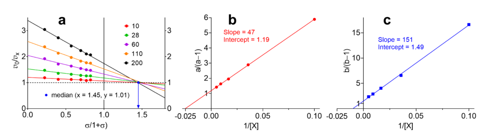
The primary plot is constructed with v0/v X as dependent variable and σ/(1+σ) as independent variable (Fig. 1). The colored solid lines in Fig. 1 represent a typical, experimentally accessible range of substrate concentrations, i.e. σ/(1+σ) from 0.2 to 0.8, corresponding to substrate concentrations from 0.2×Km to 5×Km. For practical reasons, two ordinates are drawn at the abscissa values 0 and 1.
- Independently of the mechanism, the curves of the primary plot are always straight lines
- The intercepts of the extrapolated experimental lines (dashed) on the
- 0-ordinate and the 1-ordinate are called a and b, respectively
- With the exception of the three balanced mechanisms (α = 1), for which the plot consists of lines parallel to the abscissa, the extrapolated lines of the remaining 14 mechanisms intersect at a common point with coordinates
- (α − β)/(α −1) on the abscissa and 1 on the ordinate
- The slopes are negative if α > 1 (specific or predominantly specific character)
- The slopes are positive if α < 1 (catalytic or predominantly catalytic character)
- Slopes = 0 characterize the balanced mechanisms (α = 1)
Information from the secondary plots
The values a/(a−1) and b/(b−1) are calculated and plotted against 1/[X] as shown in Figs. 2 and 3 and their expressions are
(2) ![\begin{equation*} \dfrac{{\rm{a}}}{{{\rm{a}} - 1}} = \dfrac{{\alpha {K_{\rm{X}}}}}{{\alpha - \beta }}\dfrac{1}{{\left[ {\rm{X}} \right]}} + \dfrac{\alpha }{{\alpha - \beta }} \end{equation*}](https://www.enzyme-modifier.ch/wp-content/ql-cache/quicklatex.com-464c2b00d946bbe41e8eaed55df76319_l3.png "Rendered by QuickLaTeX.com")
(3) ![\begin{equation*} \frac{{\rm{b}}}{{{\rm{b}} - 1}} = \frac{{\alpha {K_{\rm{X}}}}}{{1 - \beta }}\frac{1}{{\left[ {\rm{X}} \right]}} + \frac{1}{{1 - \beta }} \end{equation*}](https://www.enzyme-modifier.ch/wp-content/ql-cache/quicklatex.com-b76fda51eb53fdb8736413e495d02ff0_l3.png "Rendered by QuickLaTeX.com")
Properties
- The secondary plots are always straight lines
- The straight lines of both secondary plots intersect the ordinate at the common value 1 for linear inhibition mechanisms
- The straight lines of both secondary plots intersect the ordinate at values >1 for hyperbolic inhibition mechanisms
- The straight lines of both secondary plots intersect the ordinate at values <1 for nonessential activation mechanisms
- Using slopes and intercepts of the plots plots, α, β and KX can be calculated
- The value of KX can be used as initial value, while the values α and β can be constrained in the final polish by nonlinear regression analysis
The critical substrate concentration
Putting back [S]/Km into (1) in place of σ, rearranging and solving for [S], we obtain the expression (4) for the critical substrate concentration, [S]0, defined as the concentration of substrate for which the velocity is the same in the presence and in the absence of modifier
(4) ![\begin{equation*} {\left[ {\rm{S}} \right]^0} = {K_{\rm{m}}}\dfrac{{\alpha - \beta }}{{\beta - 1}} \end{equation*}](https://www.enzyme-modifier.ch/wp-content/ql-cache/quicklatex.com-9a9dc31ab29f8099db369355dcf647fd_l3.png "Rendered by QuickLaTeX.com")
Similarly, the relative critical substrate concentration is defined by (5)
(5) ![\begin{equation*} {\sigma ^0} = \dfrac{{{{\left[ {\rm{S}} \right]}^0}}}{{{K_{\rm{ m}}}}} = \dfrac{{\alpha - \beta }}{{\beta - 1}} \end{equation*}](https://www.enzyme-modifier.ch/wp-content/ql-cache/quicklatex.com-f4170ac63e6993ba04738803e44f4ec1_l3.png "Rendered by QuickLaTeX.com")
In fourteen basic modifier mechanisms α ≠ 1 and the straight lines in the specific velocity plot intersect at a common point, which represents the critical specific velocity defined as
(6) 
The critical specific velocity (6) can be measured from the specific velocity plot as the common intersection point of all straight lines. It is very useful in the diagnosis of the mechanisms and for calculating α and β.
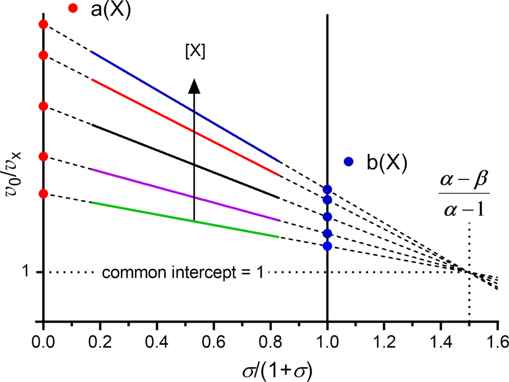
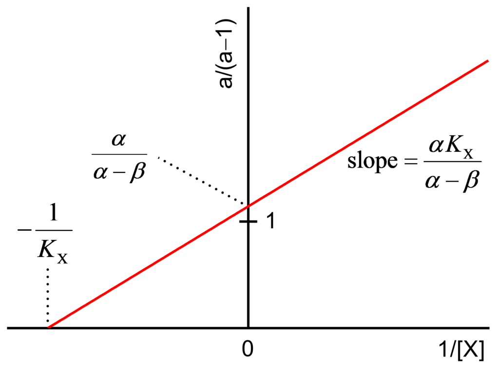
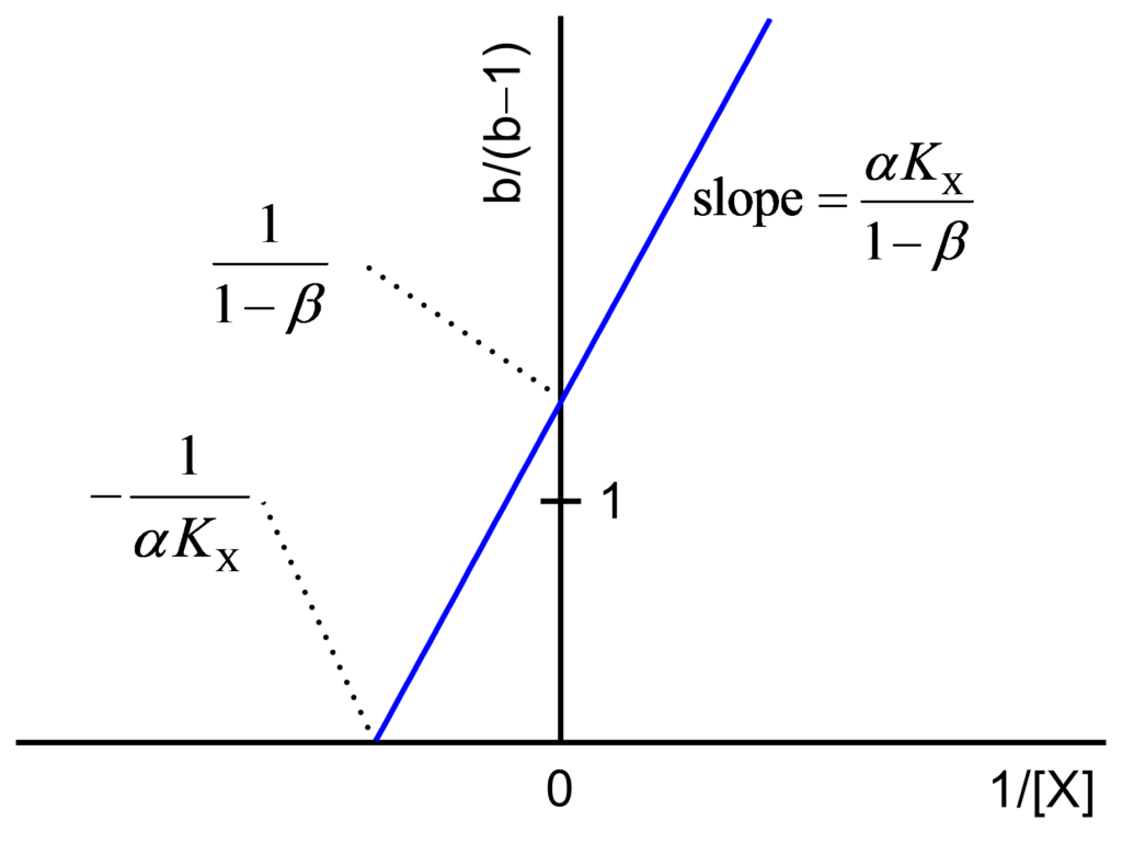
Table 1. Values/ranges of the relative critical substrate concentration and of the critical specific velocity for the basic modifier mechanisms.
| Mechanism | σ0 | σ0/(1+σ0) |
|---|---|---|
| LSpI | −∞ | 1 |
| LCaI | 0 | 0 |
| LMx(Sp>Ca)I | <0 | >1 |
| LMx(Sp<Ca)I | <0 | <0 |
| LMx(Sp=Ca)I | −1 | indeterminate |
| HSpI | indeterminate | 1 |
| HCaI | 0 | 0 |
| HMx(Sp>Ca)I | <0 | >1 |
| HMx(Sp<Ca)I | <0 | <0 |
| HMx(Sp=Ca)I | −1 | indeterminate |
| HMxD/(I/A) | >0 | (0,1) |
| HCaA | 0 | 0 |
| HMx(Sp>Ca)A | <0 | <0 |
| HMxD(A/I) | >0 | (0,1) |
| HSpA | indeterminate | 1 |
| HMx(Sp<Ca)A | <0 | >1 |
| HMx(Sp=Ca)A | 1 | indeterminate |
Table 1 lists the values or ranges of σ0 and σ0/(1+σ0) for the 17 basic modifier mechanisms. Only for mechanisms HMxD(I/A) and HMxD(A/I) the critical specific velocity falls in the experimentally accessible range. For the remaining mechanisms it is either indeterminate (division by zero) or it can be obtained by extrapolation.
In mechanism HMxD(I/A), the modifier inhibits the enzyme at [S] < [S]0, has no effect at [S] = [S]0, and activates the enzyme at [S] > [S]0. In mechanism HMxD(A/I), the modifier activates the enzyme at [S] < [S]0, has no effect at [S] = [S]0, and inhibits the enzyme at [S] > [S]0.
Warning
The specific velocity plot is a graphical diagnostic method. It should not be used for statistical purposes because σ/(1+σ) = v0/V. Therefore, errors in v0 appear in both the dependent and the independent variable invalidating regression analysis that requires stochastic independence of the two variables. Linear regression can be used to avoid subjective drawing of straight lines but without statistical rights.
In the specific velocity plot there is no whitewashing of bad data and experimental errors are shown as they are. Without inventing alternatives, repeating experiments as necessary is the best way to cure the problem. And, as already mentioned, plots that manifestly deviate from linearity may originate from inhibition or nonessential activation by the substrate itself.
Another factor is the non-adherence to the Botts-Morales general modifier mechanism and equation. If a prevailing rapid equilibrium condition does not apply, the specific velocity plot, as well as any other method based on this assumption, are pointless. However, the last case occurs only under extreme conditions analyzed in detail elsewhere [2, Chapter 2, sections 2.7 and 2.8]. Whether of not extreme deviations from the equilibrium assumption do exist can be ascertained from the dependence of Km on modifier concentration: any non-monotonous dependence , i.e. showing a maximum or a minimum, is diagnostic for this situation.
Numerical example
We consider now the same set of initial velocities used for illustrating the dependencies of kinetic parameters on modifier concentration in Raw data. First we calculate Km and V for the reaction in the absence of modifier using the velocities in the column [X] = 0 of Table 2. With these data: a) we construct the direct linear plot [3], and b) we fit the Michaelis-Menten equation (Fig. 1). Since the velocities are expressed as v/[E]t the output is kcat, not V. Both methods yield overlapping results, but for continuing our discussion we adopt the statistically-robust results from the direct linear plot, i.e. kcat = 49.8 and Km = 84.
Table 2. Initial velocities, as v/[E]t, for the numerical example
| [S] | [X] = 0 | [X] = 10 | [X] = 28 | [X] = 60 | [X] = 110 | [X] = 200 |
|---|---|---|---|---|---|---|
| 24 | 11.18 | 9.40 | 7.57 | 5.82 | 4.70 | 3.67 |
| 56 | 19.60 | 17.40 | 14.43 | 11.44 | 9.19 | 7.19 |
| 112 | 28.34 | 25.26 | 21.46 | 17.32 | 14.40 | 11.76 |
| 192 | 34.41 | 30.89 | 26.90 | 22.27 | 18.82 | 15.40 |
| 280 | 38.05 | 35.18 | 30.21 | 25.47 | 21.56 | 18.08 |
| 392 | 41.60 | 31.67 | 33.02 | 28.24 | 23.79 | 20.12 |
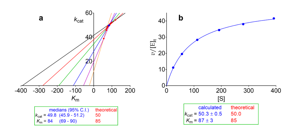
Fig 1. Calculation of kcat and Km from the initial velocities set in Table 2. (a) Direct linear plot [3] with the 95% confidence interval calculated according to [4]. (b) Fit of the Michaelis-Menten equation.
The data in Table 2 can now be transformed into those necessary for constructing the specific velocity plot, i.e. the substrate concentrations are normalized as [S]/Km and the velocities as v0/vX (Table 3). These operations are performed quickly with the help of a spreadsheet.
The specific velocity plot and the two replots are shown in Fig. 2. In the primary plot, since the data are affected by errors, the five lines do not intersect at a common point. Instead, the maximal number of possible intersect is n(n − 1)/2, where n is the number of lines, one for each modifier concentration: ten intersections in this example. (Note: a common intersection point exists only in simulations in the absence of errors, never in practice). The median of the intersection points is shown in Fig. 2a as blue dot with coordinates 1.45/1.01.
Table 3. The data in Table 2 transformed as σ/(1+σ) and v0/vX
| σ/(1+σ) | [X] = 10 | [X] =28 | [X] = 60 | [X] = 110 | [X] = 200 |
|---|---|---|---|---|---|
| 0.222 | 1.189 | 1.477 | 1.921 | 2.379 | 3.046 |
| 0.400 | 1.126 | 1.358 | 1.713 | 2.133 | 2.726 |
| 0.571 | 1.122 | 1.321 | 1.636 | 1.068 | 2.410 |
| 0.696 | 1.114 | 1.279 | 1.545 | 1.828 | 2.234 |
| 0.769 | 1.082 | 1.260 | 1.494 | 1.765 | 2.105 |
| 0.824 | 1.104 | 1.260 | 1.473 | 1.749 | 2.068 |
Calculate the parameters
With the information in Fig. 2 the sought parameters α, β, KX, and αKX can be calculated as shown in Table 4.
Recommended: The methods for calculating the parameters in red color are recommended. From several simulated sets of data with various added errors, a better estimate of αKX is obtained by multiplying α from row 9 with KX from row 3.
Important: The values of α and β can be used as known constants to be constrained in the fine-tuning procedure.
Go to The final polish, or Back to data analysis.
Table 4. Calculation of the parameters from the specific velocity plot.
| Value | Theor. | ||
|---|---|---|---|
| From the secondary plots | |||
| 1 | Slope of the a/(a−1) replot = αKX/(α−β) | 47 | |
| 2 | Ordinate intercept of the a/(a−1) replot = α/(α−β) | 1.19 | |
| 3 | KX (calculated as slope/intercept) | 39.5 | 39.8 |
| 4 | Slope of the b/(b−1) replot = αKX/(1−β) | 1.51 | |
| 5 | Ordinate intercept of the b/(b−1) replot = 1/(1−β) | 1.49 | |
| 6 | β (calculated from the intercept) | 0.33 | 0.35 |
| 7 | αKX (calculated as slope/intercept, not recommended) | 101.3 | 95.5 |
| From the primary plot and β from the intercept of the b/(b-1) replot | |||
| 8 | Critical specific velocity (α−β)/(α−1) | 1.45 | |
| 9 | Reciprocal allosteric coupling constant α | 2.49 | 2.40 |
| 10 | αKX from KX in row 3 and α in row 9 (recommended) | 98.4 | 95.5 |
Diagnosis of the mechanisms
You have constructed the specific velocity plot and secondary plots with your data and now you wish to establish to which mechanism they apply. If you have already determined the values of α and β, the mechanism can be assigned by inspection of the taxonomic tree (Fig. 3). Otherwise follow the systematic method described below.
- With your data construct the specific velocity plot and the secondary plots
- Identify in Fig. 4 the shape of the primary specific velocity plot (red numbers 1 to 12)
- Identify in Fig. 5 the shape of the two secondary plots (blue letters A to N)
- No calculations are necessary for assigning the mechanism: deduce it from Table 5.

Fig 4. The possible shapes of the primary specific velocity plot (red numbers 1 to 12). Locate the shape that matches your findings and note its number. The green arrows indicate the increasing direction of the modifier concentration.
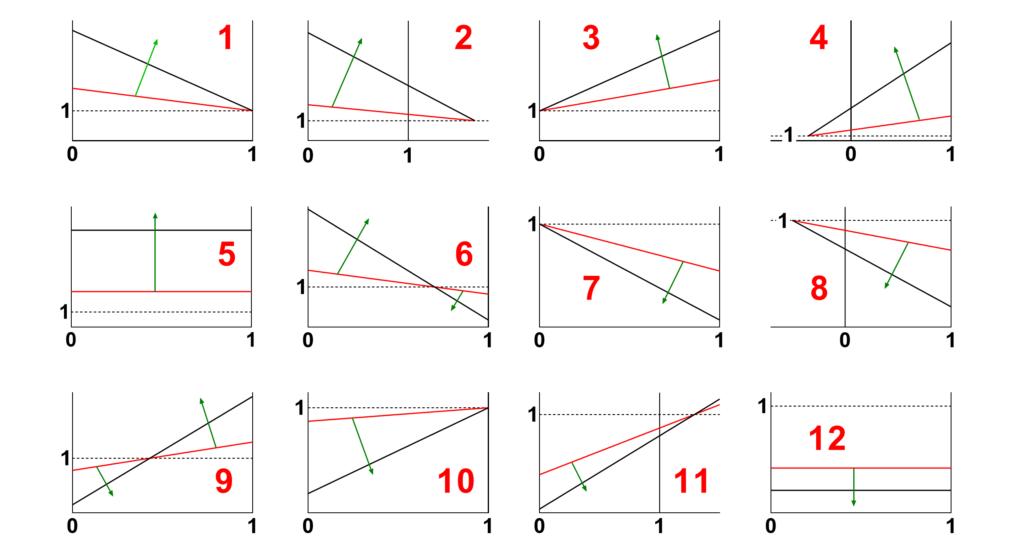
Fig. 5. The possible shapes of the secondary plots (blue letters). Locate the shape that matches your findings and note its letter.
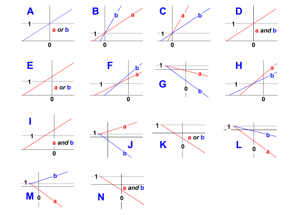
Table 5. The unique codes that identify the seventeen basic modifier mechanism according to their characteristic primary and secondary specific velocity plots. Compare your finding such as
4–C or 12–N with the codes in this table and read out the name of your mechanism.
| Acronym | Specific Velocity Plot Identification Code | Name |
|---|---|---|
| LSpI | 1-A | Linear specific inhibition |
| LCaI | 3-A | Linear catalytic inhibition |
| LMx(Sp>Ca)I | 2-B | Linear mixed, predominantly specific inhibition |
| LMx(Sp<Ca)I | 4-C | Linear mixed, predominantly catalytic inhibition |
| LMx(Sp=Ca)I | 5-D | Linear mixed, balanced inhibition |
| HSpI | 1-E | Hyperbolic specific inhibition |
| HCaI | 3-E | Hyperbolic catalytic inhibition |
| HMx(Sp>Ca)I | 2-F | Hyperbolic mixed, predominantly specific inhibition |
| HMx(Sp<Ca)I | 4-H | Hyperbolic mixed, predominantly catalytic inhibition |
| HMx(Sp=Ca)I | 5-I | Hyperbolic mixed, balanced inhibition |
| HMxD(I/A) | 6-J | Hyperbolic mixed, dual modification (inhibition → activation) |
| HCaA | 7-K | Hyperbolic catalytic activation |
| HMx(Sp>Ca)A | 8-L | Hyperbolic mixed, predominantly specific activation |
| HMxD(A/I) | 9-M | Hyperbolic mixed, dual modification (activation → inhibition) |
| HSpA | 10-K | Hyperbolic specific activation |
| HMx(Sp<Ca)A | 11-G | Hyperbolic mixed, predominantly catalytic activation |
| HMx(Sp=Ca)A | 12-N | Hyperbolic mixed, balanced activation |
Which is the mechanism of the numerical example? The primary and secondary specific velocity plots (Fig. 2) have the code 2-F. Thus the featured modification mechanism is Hyperbolic mixed, predominantly specific inhibition. If you have completed the exercise suggested in the section Raw data and explained in Concentration-dependence of parameters, your result should be the same with the code CEINP.
Download PDF: Mechanisms from the specific velocity plot
Download PDF: Fingerprints of the specific velocity plots for all mechanisms
References
- Baici A (1981) The specific velocity plot. A graphical method for determining inhibition parameters for both linear and hyperbolic enzyme inhibitors. Eur J Biochem 119: 9-14. doi:10.1111/j.1432-1033.1981.tb05570.x, PMID:7341250
- Baici A (2015) Kinetics of Enzyme-Modifier Interactions – Selected Topics in the Theory and Diagnosis of Inhibition and Activation Mechanisms. Springer, Vienna
- Eisenthal R, Cornish-Bowden A (1974) The direct linear plot. A new graphical procedure for estimating enzyme kinetic parameters. Biochem J 139: 715-720. doi:10.1042/bj1390715, PMID:4854723
- Cornish-Bowden A, Porter WR, Trager WF (1978) Evaluation of distribution-free confidence limits for enzyme kinetic parameters. J Theor Biol 74: 163-175. doi:10.1016/0022-5193(78)90069-3, PMID:713571