Well begun is half done
The procedures described here refer to the analysis of initial velocities of reversible enzymatic reactions in the presence of modifiers, in which the product concentration increases linearly with time from the beginning on the steady-state scale. Slow-onset inhibition mechanisms, characterized by progress curves consisting by one-two exponential phase(s) followed by a linear steady-state, are not yet treated in this website, but are considered in due detail [1], Chapter 8.
Performing data analysis without prior identification of the mechanism, i.e. by fitting a set of equations to raw data and selecting the best fitting model on the basis of its superior statistical tests with respect to the other models, may fail to identify the true mechanism. One of the equations may perform better than the others even if the winning model is wrong or incomplete and two or more parameters are intertwined to the point to invalidate their calculated values. Conversely, a mechanism should be determined first without prejudice: the shapes of diagnostic plots are sufficient to assign a mechanism unequivocally. With this, one or more parameters can be constrained in the final refinement of the remaining parameters by regression analysis.
Know the rules first, then play the game
Technical points and practical suggestions
It is advisable that beginners in enzyme kinetics, not yet familiar with the basic theories of enzyme-modifier interactions, gather the necessary information before starting their experiments. Mostly important is to become conversant with the palette of existing mechanisms described under Mechanisms. For readers interested in deepening this topic, the necessary material is assembled in [1], Chapters 1-3, with numerous examples of published work annotated in Chapter 5.
The amount of raw data necessary for identifying a mechanism with high probability and calculating statistically meaningful parameters depends on the complexity of the mechanism itself. When used in regression analysis, the corresponding rate equation, which contains all parameters of the system, performs badly unless an adequate number of data points is available.
When one or more modifiers are studied, for instance a series of new compounds identified by high-throughput docking procedures and supposed to behave as inhibitors of a given enzyme, their properties are still unknown. Trying to identify a mechanism with a few substrate concentrations at two fixed modifier concentrations might just be sufficient to obtain a crude estimate of the type of mechanism concerned. Pretending that this approach establishes the mechanism and affords trustful parameters belongs however to the realm of fantasy.
- Careful design of the experiment. The number and sequence of the planned measurements, dilutions, pipetting schemes, preincubation of reagents, etc. are best laid down ahead.
- Temperature control of all reagents within ±1°C. In enzyme kinetics, the room temperature does not exist.
- Buffer composition, concentration of the buffering species, pH with two significant decimals (e.g. pH 7.40), ionic strength, buffer capacity, temperature coefficient (change of pH with temperature) must be controlled precisely.
- Organic solvents, if added, should be maintained at a constant concentration in all experiments, including blanks.
- Enzyme stability. The Selwyn-test [1, pp. 45-51] is a handy method to monitor any loss of enzyme activity during the measuring time. This problem may be irrelevant when measuring initial velocities over a short time.
- Initial velocities measured as precisely as possible are a key element of steady-state kinetics. Their quality depends on the detection method that can be continuous or discontinuous. The segment method for measuring the initial velocity is a boring approach that can, however, be almost fully automated using a spreadsheet [1, pp. 51-59].
Tutorial with a numerical example
Table 1 shows a set of initial velocities at six concentrations of the varied substrate in the absence of and at five fixed concentrations of a modifier whose kinetic properties are not yet revealed. All other reactants are present at fixed, constant concentrations. These data are shown as filled circles in Fig. 1 with a different color for each modifier concentration. The ‘data’ were simulated using the complete steady-state rate equation without making any simplifying assumption and adding a multiplicative random error of 1.2% standard deviation of the calculated rates (details in [1, Chapter 2]). The same data will be used in this and in the two following pages.
Under prevailing equilibrium conditions, the rate equation of the general modifier mechanism (1) (see in the Methods section (Inhibition and nonessential activation), can be rewritten and rearranged as follows:
(1) ![\begin{equation*} \dfrac{\ratev}{{{{\left[ {\rm{E}} \right]}_{\rm{t}}}}} = \dfrac{{{k_2}\left( {1 + \beta \dfrac{{\left[ {\rm{X}} \right]}}{{\alpha {K_{\rm{X}}}}}} \right)\left[ {\rm{S}} \right]}}{{{K_{\rm{m}}}\left( {1 + \dfrac{{\left[ {\rm{X}} \right]}}{{{K_{\rm{X}}}}}} \right) + \left[ {\rm{S}} \right]\left( {1 + \dfrac{{\left[ {\rm{X}} \right]}}{{\alpha {K_{\rm{X}}}}}} \right)}} \end{equation*}](https://www.enzyme-modifier.ch/wp-content/ql-cache/quicklatex.com-e0ea564949628c370babdcce684728b3_l3.png "Rendered by QuickLaTeX.com")
Further rearrangement as (2) reveals the apparent values of kcat and Km, shown in red and blue, respectively:
(2) ![\begin{equation*} \dfrac{\ratev}{{{{\left[ {\rm{E}} \right]}_{\rm{t}}}}} = \dfrac{{{k_2}\dfrac{{1 + \beta \dfrac{{\left[ {\rm{X}} \right]}}{{\alpha {K_{\rm{X}}}}}}}{{1 + \dfrac{{\left[ {\rm{X}} \right]}}{{\alpha {K_{\rm{X}}}}}}}\left[ {\rm{S}} \right]}}{{{K_{\rm{m}}}\dfrac{{1 + \dfrac{{\left[ {\rm{X}} \right]}}{{{K_{\rm{X}}}}}}}{{1 + \dfrac{{\left[ {\rm{X}} \right]}}{{\alpha {K_{\rm{X}}}}}}} + \left[ {\rm{S}} \right]}} \end{equation*}](https://www.enzyme-modifier.ch/wp-content/ql-cache/quicklatex.com-10dd0a502d6148627aa4a1ae1f4cce4c_l3.png "Rendered by QuickLaTeX.com")
(3) ![\begin{equation*} \textcolor{red}{k_{{\rm{cat}}}^{{\rm{app}}} = {k_2} \times \frac{{1 + \beta \dfrac{{\left[ {\rm{X}} \right]}}{{\alpha {K_{\rm{X}}}}}}}{{1 + \dfrac{{\left[ {\rm{X}} \right]}}{{\alpha {K_{\rm{X}}}}}}}} \end{equation*}](https://www.enzyme-modifier.ch/wp-content/ql-cache/quicklatex.com-d04d7c26a4354beff51778a22f47ca0f_l3.png "Rendered by QuickLaTeX.com")
(4) ![\begin{equation*} \textcolor{blue}{K_{\rm{m}}^{{\rm{app}}} = {K_{\rm{m}}} \times \dfrac{{1 + \dfrac{{\left[ {\rm{X}} \right]}}{{{K_{\rm{X}}}}}}}{{1 + \dfrac{{\left[ {\rm{X}} \right]}}{{\alpha {K_{\rm{X}}}}}}}} \end{equation*}](https://www.enzyme-modifier.ch/wp-content/ql-cache/quicklatex.com-987b677b8766afec02d167e2dc80ff40_l3.png "Rendered by QuickLaTeX.com")
In its condensed form (5), equation (2) is indispensable for nonlinear fitting purposes of raw data. In fact, the apparent kcat and Km values contain all necessary information for determining the mechanism and calculating the sought parameters.
(5) ![\begin{equation*} \dfrac{\ratev}{{{{\left[ {\rm{E}} \right]}_{\rm{t}}}}} = \dfrac{{k_{{\rm{cat}}}^{{\rm{app}}}\left[ {\rm{S}} \right]}}{{K_{\rm{m}}^{{\rm{app}}} + \left[ {\rm{S}} \right]}} \end{equation*}](https://www.enzyme-modifier.ch/wp-content/ql-cache/quicklatex.com-4ed80f85d9d6824e181710066a3da339_l3.png "Rendered by QuickLaTeX.com")
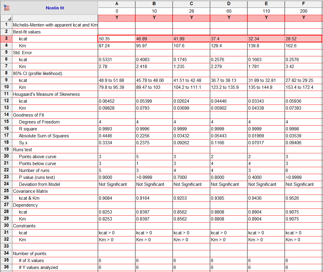
Equation (5) is now fitted to the data in Fig. 1 by nonlinear regression to extract the apparent values of kcat and Km. The solid lines in Fig. 1 represent best-fits from this procedure, while Table 2 contains the results obtained with GraphPad Prism software [2]. As other similar software, besides graphics, this package offers an ample choice of statistical tests some of which were used in this example.
Try yourself
Download Raw data_Table 1 , elaborate the data with your preferred software as described in this page, and compare your results with those in Table 2.
Data
Table 1. Raw data the initial velocities in Fig. 1 as v/[E]t
| [S] | [X] = 0 | [X] = 10 | [X] = 28 | [X] = 60 | [X] = 110 | [X] = 200 |
|---|---|---|---|---|---|---|
| 24 | 11.18 | 9.40 | 7.57 | 5.82 | 4.70 | 3.67 |
| 56 | 19.60 | 17.40 | 14.43 | 11.44 | 9.19 | 7.19 |
| 112 | 28.34 | 25.26 | 21.46 | 17.32 | 14.40 | 11.76 |
| 192 | 34.41 | 30.89 | 26.90 | 22.27 | 18.82 | 15.40 |
| 280 | 38.05 | 35.18 | 30.21 | 25.47 | 21.56 | 18.08 |
| 392 | 41.60 | 31.67 | 33.02 | 28.24 | 23.79 | 20.12 |
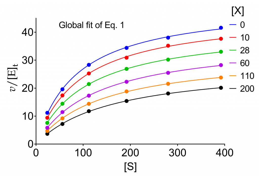
Table 2. Results of fitting equation (5) to the data in Fig. 1 using GraphPAD Prism software. Zoom/Download
We inspect now the dependencies of the kinetic parameters on modifier concentration. kcatapp and Kmapp taken from Table 2 are used to calculate (1/kcat)app, (kcat/Km)app, and (Km/kcat)app (Table 3). The data are plotted below as a function of modifier concentration and commented. These plots are useful for the preliminary calculation of the kinetic parameters (this page) and for performing a systematic diagnosis of the kinetic mechanism of the modifier (Concentration dependence of parameters).
Table 3. Kinetic parameters and derived expressions.
| [X] = 0 | [X] = 10 | [X] = 28 | [X] = 60 | [X] = 110 | [X] = 200 | |
|---|---|---|---|---|---|---|
| kcatapp | 50.35 ± 0.53 | 46.89 ± 0.41 | 41.99 ± 0.17 | 37.40 ± 0.26 | 32.34 ± 0.17 | 28.52 ± 0.26 |
| Kmapp | 87.24 ± 2.78 | 95.97 ± 2.42 | 107.6 ± 1.23 | 129.4 ± 2.28 | 139.8 ± 1.78 | 162.6 ± 3.42 |
| 1/kcatapp | 1.99 × 10⁻² | 2.13 × 10⁻² | 2.38 × 10⁻² | 2.67 × 10⁻² | 3.09 × 10⁻² | 3.51 × 10⁻² |
| (kcat/Km)app | 0.58 | 0.49 | 0.39 | 0.29 | 0.23 | 0.18 |
| (Km/kcat)app | 1.73 | 2.05 | 2.56 | 3.46 | 4.31 | 5.70 |
Dependence of the kinetic parameters on [X] and preliminary calculations
What follows below is just to illustrate how preliminary information from raw data can be obtained before applying more precise approaches. As discussed further down, access to a trustworthy determination of the basic modifier mechanism and associated kinetic parameters is straightforward and effortless.
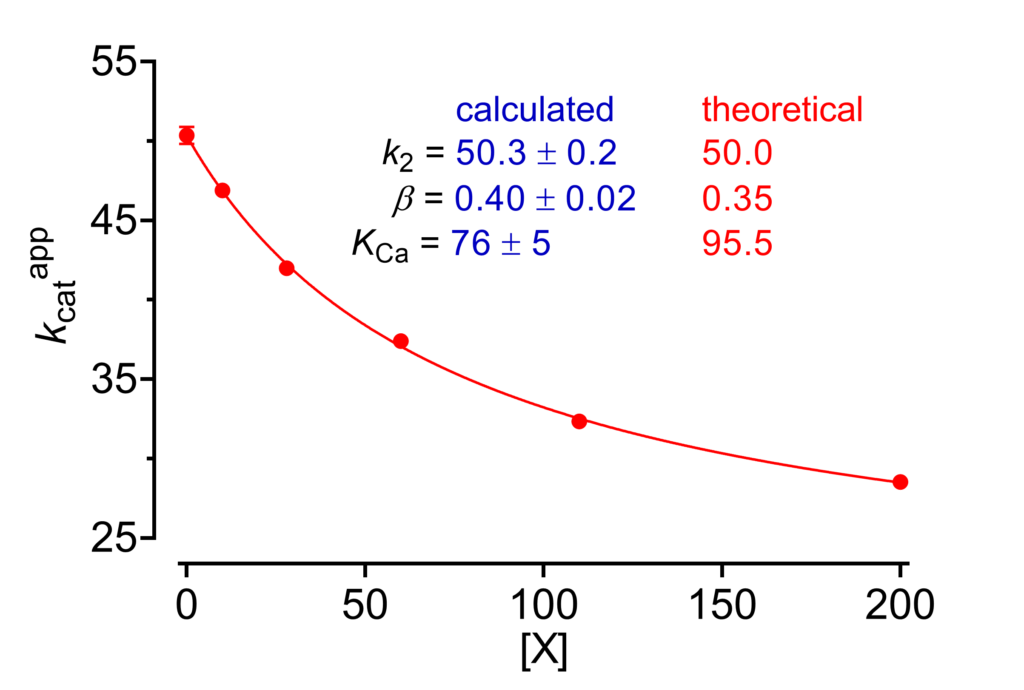
kcatapp against [X]
We begin from the plot of kcatapp against [X] (Fig. 2). In the expression of this parameter (6) α and KX can obviously not be separated but we can consider ‘αKX‘ as the equilibrium dissociation constant, KCa, of the catalytic component of the general modifier mechanism.
(6) ![\begin{equation*}k_{{\rm{cat}}}^{{\rm{app}}} = {k_2} \times \dfrac{{1 + \beta \dfrac{{\left[ {\rm{X}} \right]}}{{\alpha {K_{\rm{X}}}}}}}{{1 + \dfrac{{\left[ {\rm{X}} \right]}}{{\alpha {K_{\rm{X}}}}}}} \equiv {k_2} \times \frac{{1 + \beta \dfrac{{\left[ {\rm{X}} \right]}}{{{K_{{\rm{Ca}}}}}}}}{{1 + \dfrac{{\left[ {\rm{X}} \right]}}{{{K_{{\rm{Ca}}}}}}}}\end{equation*}](https://www.enzyme-modifier.ch/wp-content/ql-cache/quicklatex.com-b3bd71713ddc99cb5c8e0739d3026087_l3.png "Rendered by QuickLaTeX.com")
Equation (6) can be fitted to data to calculate k2, β and KCa (Fig. 2). As discussed in [1, Chapter 2], the probability that the calculated parameters are close to their true values is high for k2, satisfactory for β, while KCa may suffer from some bias. This plot is powerful in combination with the other plots discussed in this page.
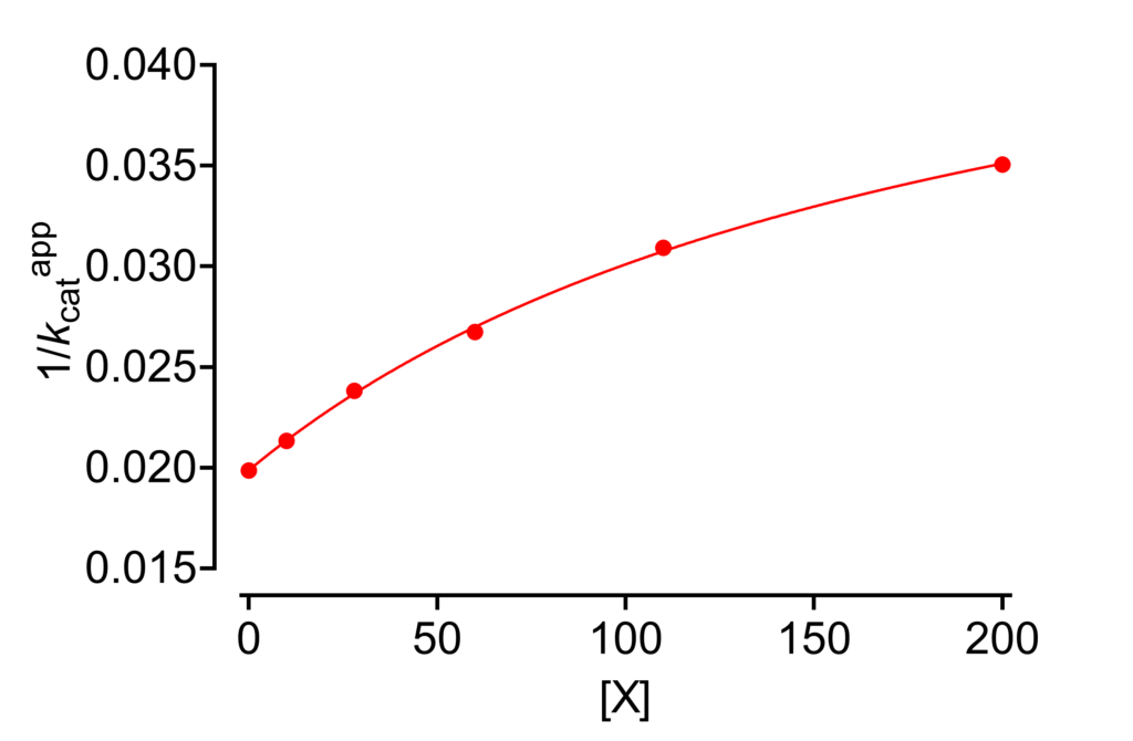
1/kcatapp against [X]
As far as the parameters are concerned, the dependence of 1/kcatapp on [X] gives the same information as the preceding plot. Its main purpose is a diagnostic one when used together with other plots for assessing the mechanism. The plot of 1/kcatapp against [X] is shown in Fig. 3.
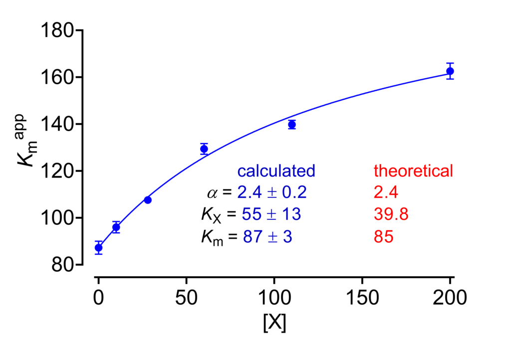
Kmapp against [X]
The dependence of Kmapp on [X] is descried by equation (4) above. The fit of this equation to data affords good estimates of α and Km, while KX is determined with some uncertainty [1, Chapter 2].
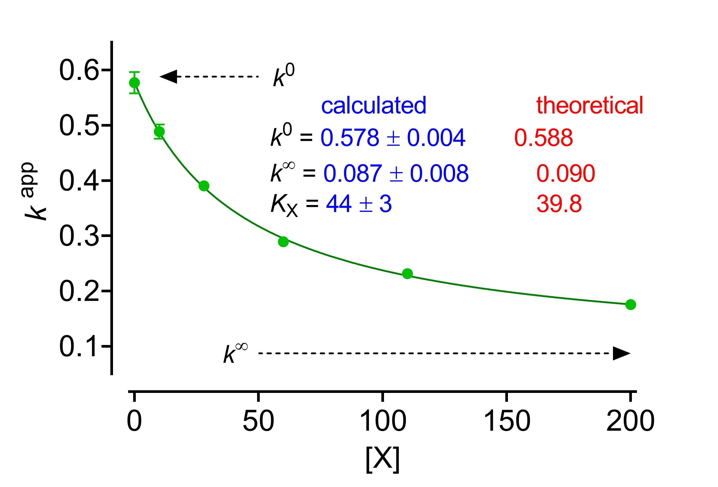
(kcat/Km)app against [X]
The expression of the specificity constant is
(7) ![\begin{equation*} {\left( {\dfrac{{{k_{{\rm{cat}}}}}}{{{K_{\rm{m}}}}}} \right)^{{\rm{app}}}} = \dfrac{{{k_2}}}{{{K_{\rm{m}}}}} \times \dfrac{{1 + \beta \dfrac{{\left[ {\rm{X}} \right]}}{{\alpha {K_{\rm{X}}}}}}}{{1 + \dfrac{{\left[ {\rm{X}} \right]}}{{{K_{\rm{X}}}}}}} \end{equation*}](https://www.enzyme-modifier.ch/wp-content/ql-cache/quicklatex.com-c819c08671c347b91dbb5be5e1283649_l3.png "Rendered by QuickLaTeX.com")
Fitting 7 to data is problematic because it contains 5 parameters, some of which are intertwined, but satisfactory solutions are available [1, Chapter 2]. One of these, proposed by Di Cera et al. [3], considers that, increasing [X], the specificity constant varies between its value at [X] = 0 (k 0) and [X] = ∞ (k∞), where k = kcat/Km:
(8) ![\begin{equation*} {k^{{\rm{app}}}} = \dfrac{{{k^0} + {k^\infty }\dfrac{{\left[ {\rm{X}} \right]}}{{{K_{\rm{X}}}}}}}{{1 + \dfrac{{\left[ {\rm{X}} \right]}}{{{K_{\rm{X}}}}}}} \end{equation*}](https://www.enzyme-modifier.ch/wp-content/ql-cache/quicklatex.com-ef8b286121c149849abe110817ca587f_l3.png "Rendered by QuickLaTeX.com")
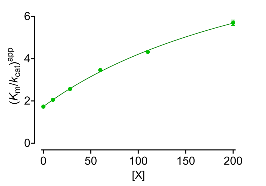
(Km/kcat)app against [X]
Equation (8) is certainly better suited for calculating the kinetic parameters with respect to its reciprocal counterpart. Nevertheless, the dependence of the reciprocal specificity constant on modifier concentration (Fig. 6) is diagnostically useful when used together with the other plots shown above for identifying the pertinent basic modifier mechanism among seventeen possibilities (see Fig. 1 in Inhibition and nonessential activation).
Back to Data Analysis or go directly to Concentration-dependence of parameters to learn an easy and powerful discrimination method between the basic mechanisms of enzyme modification.
References
- Baici A (2015) Kinetics of Enzyme-Modifier Interactions – Selected Topics in the Theory and Diagnosis of Inhibition and Activation Mechanisms. Springer, Vienna.
- GraphPad Prism version 7.00 for Windows, GraphPad Software, La Jolla California USA, www.graphpad.com
- Di Cera E, Hopfner KP, Dang QD (1996) Theory of allosteric effects in serine proteases. Biophys J 70: 174-181.